Tutorial: the gradient

The gradient is a field in which every device holds its distance from the nearest source. It needs nothing but local state and neighbor exchanges, yet it has a global meaning, and it is the building block of most other patterns: broadcast, collect_with and elect_leaders are all built on top of it.

The complete code, including the script that produced the animations, is in docs/examples/gradient.py.

1. Each device remembers its estimate

A device cannot know its distance in one shot: it keeps an estimate and refines it at every round. State that survives across rounds is remember (the rep of field calculus). Before knowing anything, the estimate is infinity:

set_distance, distance = remember(float("inf"))

2. Look at the neighbors' estimates

neighbors(distance) sends the local estimate to the neighbors and returns a NeighborhoodField: one value per neighbor, plus the device itself. Arithmetic on fields is element-wise, so + 1 adds one hop to each neighbor's estimate, giving the distance through that neighbor:

through_neighbors = neighbors(distance) + 1

3. Keep the best one

A source is at distance 0; any other device takes the shortest path its neighbors offer. exclude_self() drops the device's own entry, so that it cannot lean on itself:

@aggregate
def hop_gradient(source: bool) -> float:
    """Number of hops to the nearest source, built from remember and neighbors."""
    set_distance, distance = remember(INFINITY)
    through_neighbors = neighbors(distance) + 1
    nearest = min(through_neighbors.exclude_self().values(), default=INFINITY)
    set_distance(0 if source else nearest)
    return distance

Read locally, it compares a few numbers. Read globally, it is a distributed shortest-path algorithm: round after round the correct distances spread from the source, until the whole network holds its hop count.

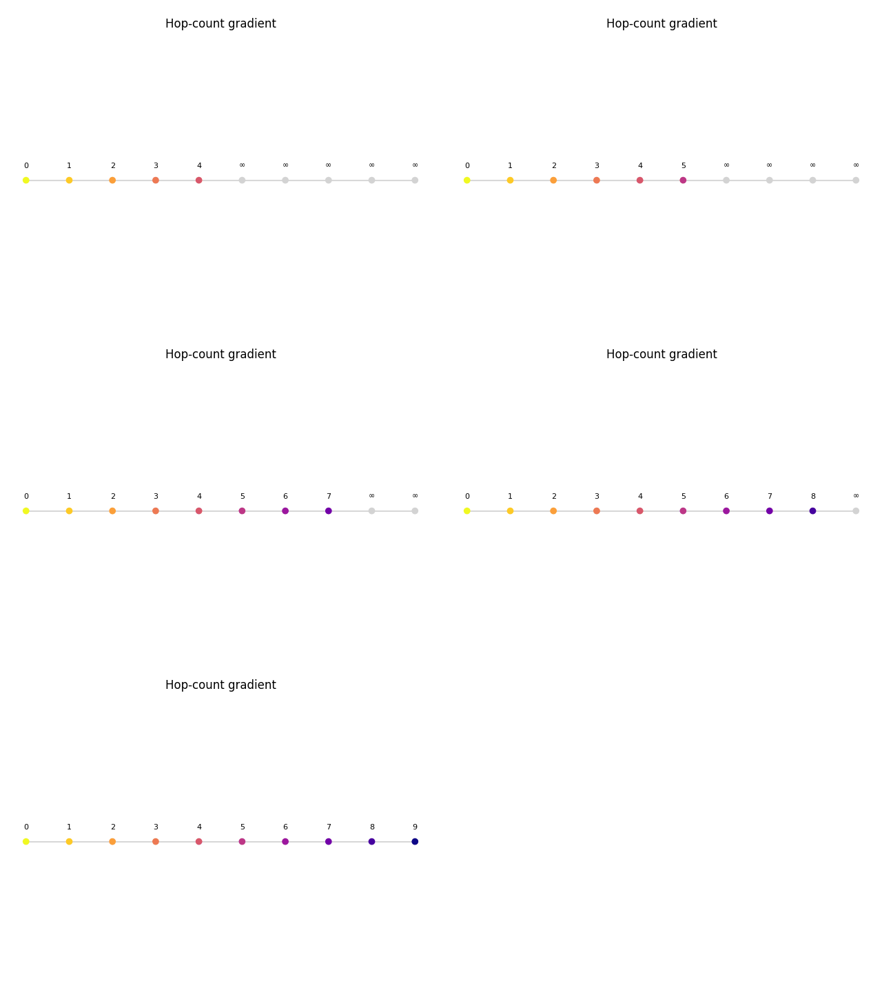
Why does the wave move more than one hop per round?

In the phyelds simulator the devices of one round run one after the other and read the freshest messages of the neighbors that already ran. The final field does not depend on that order; only the speed does.

4. Run it

Every device runs the same program, and reads whether it is a source from a sensor. The simulator provides the deployment, the neighborhood relation and the scheduling:

from phyelds.calculus import aggregate
from phyelds.libraries.device import sense
from phyelds.simulator import Simulator
from phyelds.simulator.deployments import grid_generation
from phyelds.simulator.neighborhood import radius_neighborhood
from phyelds.simulator.runner import schedule_program_for_all

@aggregate
def program():
    return hop_gradient(sense("source"))

simulator = Simulator()
grid_generation(simulator, width=10, height=1, spacing=1.0)   # a line of 10 devices
simulator.environment.set_neighborhood_function(radius_neighborhood(1.1))
simulator.environment.add_data_for_all_nodes({"source": False})
simulator.environment.nodes[0].data["source"] = True          # device 0 is the source

schedule_program_for_all(simulator, start=0.0, frequency=1.0, program=program)
simulator.run(12)
print([node.data["result"] for node in simulator.environment.nodes.values()])
# [0, 1, 2, 3, 4, 5, 6, 7, 8, 9]

5. From hops to distances

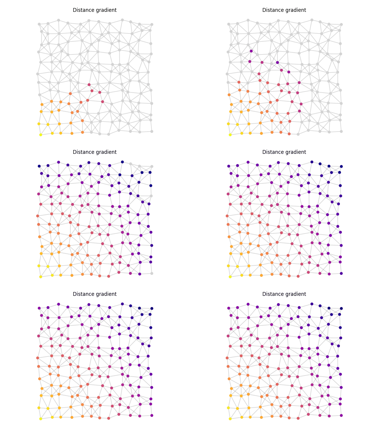
Replacing the constant 1 with the measured distance to each neighbor gives a metric gradient. That is what the library distance_to does:

from phyelds.libraries.distances import neighbors_distances
from phyelds.libraries.spreading import distance_to

@aggregate
def program():
    return distance_to(sense("source"), neighbors_distances())

Run it in the playground

6. Self-healing

Nothing in the program refers to when the source appeared or where it is: every round recomputes the field from the current state of the network. When the source jumps to the opposite corner, the field repairs itself with no extra code.

Run it in the playground

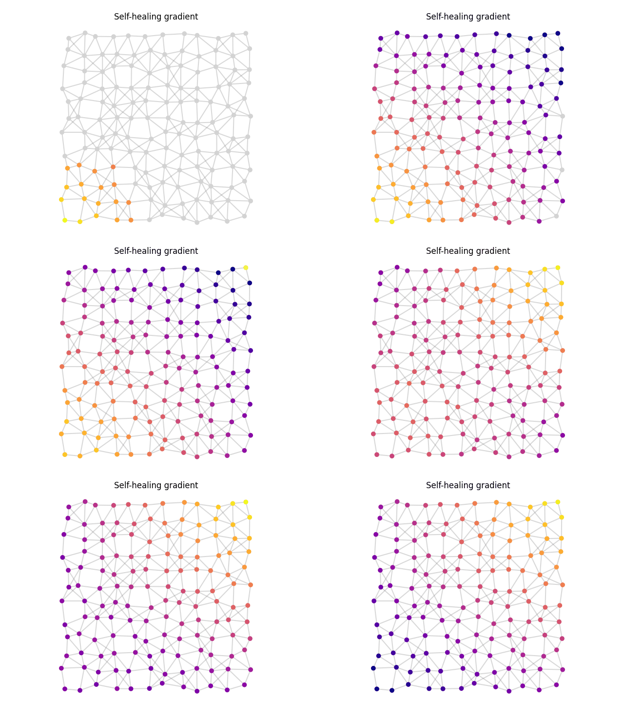
The area around the new source settles quickly; the old one is slower, because its devices can only raise their stale, too-small estimates a little at a time, leaning on each other. This is the rising value problem of the classic gradient: see Pitfalls.

Where next

• Aggregate programs: the execution model behind what you just ran.
• Libraries: broadcast, collection, gossip and leader election, all built on gradients.